I. Introduction
Housing price has been our society’s constant interest in recent years, and has been recognized as an important economic factor that has a close relation to individuals, policy-making authorities, and financial institutions. First of all, housing assets form a great part (68%)1) of Korean people’s personal wealth. Mills (2008) showed that housing business is a critical factor in a close relation to a country’s economy from the viewpoint of policy-making authorities, citing that 20 housing business recessions between 1970 and 2000 led to 19 economic recessions in OECD countries. Crawford (1995) showed that housing price volatility is a major factor behind mortgage default and loan prepayment, and is particularly very important to financial institutions heavily relying on housing mortgage loans. That is, it may be said that housing price is an important factor in terms of the stabilization of national economy at large and relevant policy-making, not merely in terms of housing economy.
Studies on housing price prediction has significance in that they reduce uncertainty about future housing price and derive related policy implications. Accordingly, a number of researchers and research institutions have suggested a variety of research models and methodologies, attempting to develop econometric models that can reduce the error range by means of simpler structure. However, the VAR model and the ARIMA model, traditional econometric approaches used in the existing studies, have two structural limitations. First, because of the trade-off relation between forecasting performance and analysis structure, if housing price prediction variables increase and are diversified, a problem occurs that while forecasting performance increases, the analysis structure becomes complicated at the same time. This not only makes analysis more difficult, but also can cause the overfitting problem that rather reduces analytic power.
In addition, the existing methodologies have limitations in the improvement of forecasting performance because they can’t reflect the uncertainty of models themselves in advance. That is, in case of starting analysis with a specific model in which a researcher’s subjectivity is reflected, uncertainty inherent in the model makes it difficult to make a more elaborate prediction.
In consideration of the problems, this study has the following two main objectives. First, it intends to derive a research model capable of resolving the problem of model complexity and improving the forecasting performance, by using the Bayesian methodology, not the existing approaches. The Bayesian model selection (BMS) and the Bayesian model averaging (BMA), which are based on Bayesian theories, not only allow analysis that reflects the uncertainty of a model, but also have strengths in the improvement of forecasting performance because they use more information than the existing methodologies. Thus, this study will select a better prediction model after comparing actual measurement values with an apartment trade price index estimated by using the above Bayesian analysis methodologies and an apartment trade price index estimated with the AR model mostly used in the existing analyses.
In addition, this study intends to derive analysis results that reflect regional characteristics, by selecting different regions as its analysis targets for the diversification of its analysis targets. The degree and size of changes in real estate prices such as the apartment price vary according to the environmental factors of regions as well as the macroeconomic or policy factors of a nation. Like this, regional differences can be viewed as very important judgment factors in analysis, and this study will select two regions of Seoul and Busan, and show analysis results suitable to each of them.
II. Previous Studies
The purpose of housing price studies is to explain causes of housing price fluctuation and analyze major determinants or to predict future housing price on the basis of the theoretical background. In particular, awareness about the importance of housing price and the fluctuation of housing price, which was formed after the United States sub-prime mortgage crisis, raised the necessity for new understanding and approach towards housing price; and a lot of studies have suggested alternatives, using diverse analysis methods.
Housing price is determined by the effects of diverse factors such as the hedonic characteristics of individual houses, a country’s policies and macroeconomic factors, supply and demand conditions, and regional economic factors. The hedonic characteristics of housing price refer to unobserved characteristics inherent in housing; and the existing studies analyzed their correlations with housing price and their effects, using various factors such as right to site, geographical characteristics, the component ratios of land and building, floor area ratio, prospect right, southern exposure, and school district (Lim Byung-koon, 2006; Jung Sung-yong, 2009). The hedonic price models of housing price, however, have structural limitations in variable category selection, model development, and model estimation as well as data acquisition (Lee Young-man, 2008). Particularly, heteroscedasticity caused by regional characteristics and the problem of omitted variables that may occur during variable selection can lead to distorted results, and thus careful analysis is required. On this, Youn Hoo- mug et al. (2013) have shown that the regional characteristics of housing have greater influence than its individual characteristics, compared with the past, by analyzing housing price in Seoul with a hierarchical linear model.
In connection with housing policies, using quantified real estate policy as policy variable, Choi Cha-soon (2010) showed that the real estate policy has causal relationship with the fluctuation of real estate price, and that responses to the policy vary with regions, apartment and lease markets, and land sales markets. And Ham Jong-young et al. (2012) emphasized the endogeneity problem of the policy variable, given that the real estate policy and the market trends don’t form causality in the short term. From the multiple regression analysis, Noh Young-hak et al. (2012) drew the conclusion that the housing price index is greatly influenced by macroeconomic variables, particularly, the composite leading index and the composite stock price index, rather than housing-related policies, but exposed the limitation of being rather unrealistic because they failed to reflect market instability that occurs during changes in government. On this wise, to analyze the effects of a housing policy properly, the problem occurs that various factors such as endogeneity as well as elaborate modeling considering time, region, and market should be taken into consideration.
Socioeconomic variables in housing price studies usually consist of economic variables on the national level such as GDP, the unemployment rate, the consumer price index, and the market interest, and economic variables on the regional level such as the fluctuation rate of land price and trade performance. First, in connection with macroeconomic variables, Dolde and Tirtiroglu (2002) showed that housing price is related to the variables of revenue increase, inflation, and interest rate. And Kim Hyun-jae (2011) suggested the findings that variables like unemployment also have effects on housing price. That is, socioeconomic factors are very important in housing price analysis; and thus, in studies of more diverse regions, socioeconomic variables on the national level or the regional level are mainly used.
The effects of macroeconomic variables, however, appear differently according to time and regions. In analyses with periods divided into before and after the currency crisis and the financial crisis, Kim Yun-yeong (2012) showed that macroeconomic variables have significant effects on housing price. And Han Kyung-soo (2011) derived the results that the effects of macroeconomic variables on housing price vary with regions. This implies that in housing price analysis, macroeconomic variables and regional factors should be considered over various periods, and that such differences in effects cause difficulty in analysis and model selection.
Housing price forecasting studies predict future housing price, using time series analysis, on the basis of the fact that housing price fluctuates depending on past prices. Thus, in the existing studies, attempts were made to derive models that show better forecasting performance by comparing the error ranges of models such as VAR and ARIMA (Case and Shiller, 1989; Lee Young-soo, 2014). In a study that comparatively analyzed ARMA and VAR, Son et al. (2003) compared and analyzed a VAR model and an ARMA model, real estate price prediction models that considered the real GDP growth rate and the rate of return on corporate bond, and showed that the forecasting performance the VAR is excellent. Son Jung-shik et al. (2002) constructed a VAR prediction model with macro variables that were theoretically consistent and were found to be significant in causality analysis, and attempted to analyze a new real estate price prediction model that reflected changes in market conditions; and as a result, they drew the conclusion that the VAR model is comparatively excellent than the ARMA model. A study on apartment housing price index forecasting models, a similar study carried out by Korea Housing Finance Corporation (2012), found that ARMA is better than VAR in terms of the minimization of prediction error, whereas VAR, which reflects macroeconomic variables, is better during a period of a sharp fluctuation in the housing business.
Like this, it was found that the existing models had their own advantages and disadvantages according to circumstances, but still showed limitations in forecasting performance. Hence, new forecasting models were proposed to remedy the problem. First, as for housing price forecasting studies using ARMA, Kim (1998) and Yoon Ju-hyun et al. (2000) compared and analyzed the results of ARMA models and state space models, models for the short-term prediction of housing price, and drew the conclusion that the state space model is better than the ARMA model in terms of forecasting performance. Lee and Lee (2009) analyzed the housing price index of Seoul Metropolitan City by using ARMA and artificial neural network models, and found that there was no statistically significant difference between the two models, but the artificial neural model was better than the ARMA model in terms of predictability. Findings of a study, which compared the housing price forecasting performance of univariate time series models including an ARMA model, an IGARCH model, a regime-switching (RS) model, and an unobserved-component (UC) model, showed that in the case of out-of-sample forecasts, the forecasting performance of the unobserved-component model was far lower than that of the regime-switching model (Lee Young-soo, 2014).
Further, Bayesian Model Selection (BMS) and Bayesian Model Averaging (BMA), which are based on Bayesian theories, not traditional statistical approaches, are attracting attention as methodologies that improved the problem of uncertainty in model selection. BMS and BMA models were first introduced by Bates and Granger (1969), and their predictability has since been proved by a variety of studies. In particular, the BMA model was used in time-series analysis studies to forecast inflation (Engle, Granger and Kraft, 1984; Wright, 2008), money supply (Figlewski and Urich, 1983), the exchange rate (Bilson, 1983), and the GDP growth rate (Fernández et al., 2001). And in connection with housing price forecasting, it was used in a variety of empirical analyses on the United States (Dua et al., 1999), Switzerland (Stadelmann, 2010), South Africa (Gupta et al., 2008), and so on.
Hence, this study intends to derive a housing price prediction model, using BMS and BMA that consider uncertainty in model selection.
III. Data and Analysis
As an indicator for the prediction of housing price, this study selected the apartment sale price index for Seoul and Busan, which is prepared and published every month by the Korea Appraisal Board on the basis of apartment sale price data. The apartment sale price index is a value of volatility calculated based on data on the sale prices of the same apartments that reported two or more transactions during a period of index calculation, with January 2006 as the reference period (100). It is widely used in that it provides exact information on market trends by investigating the level and volatility of apartment trade prices; fundamentally, however, it has two serious problems in its calculating method. First, there is a problem of inefficiency in data use that occurs in case the sale price of the same apartment is not observed repeatedly. If the sale price of the same condition is not observed repeatedly, the relevant data is excluded from index calculation, which may result in negative effects on the stability of the price index. Second, there is a problem of sampling error that occurs because price data on apartments of the perfectly same size in the same apartment complex can’t be obtained at every time period. Consequently, sampling bias caused by differences in the frequency of apartments observed at every period occurs, and can act as a factor that lowers the reliability of the index. In this connection, Lee Chang-moo et al. (2008) re-calculated the apartment sale price index, which reflects sale price data excluded by the existing methods of repeat sales index calculation, in order to solve the above problems by using both transaction prices and asking prices that represent apartment value; and as a result, showed that the improvement of about 18.6% in data utilization was possible. However, although this approach showed great effects in terms of the efficiency of data utilization, it was found that it failed to show any great difference in the changes of the apartment sale price index. Therefore, this study did not re-calculate a separate apartment sale price index, but used the apartment sale price index disclosed by the Korea Appraisal Board, as it was, without any modification.
As for independent variables, a total of 11 macroeconomic indicators and real estate-related indices provided by the Statistics Korea and the Bank of Korea from January 2007 to December 2014, including the fluctuation rate of land price, the employment rate, the apartment construction performance, the apartment trading status, the consumer price index, the market interest, the mortgage rate, GDP (real and nominal), the index of all industry production, and the CD rate, were used. The above independent variables largely consist of supply variables and demand variables. First, the supply variables are variables that influence the apartment sale price from the side of apartment supply; and include the apartment construction performance, which reflects the effects of construction business, and the fluctuation rate of land price, which reflects the price volatility of land needed for apartment construction. On the other hand, the demand variables are variables that influence the apartment sale price from the side of apartment demand; and the apartment trading status, the unemployment rate, the consumer price index, the market interest, the mortgage rate, GDP (real and nominal), the index of all industry production, and the CD rate were selected as them. Overall, GDP, the consumer price index, the index of all industry production, the unemployment rate, and the CD rate were used to reflect the effects of income or the movement of market interest; and the mortgage rate was additionally used on the basis of the findings of a study on positive relationship between house prices and bank lending (Park Yun-woo et al., 2012). Among the above variables, the fluctuation rate of land price, the unemployment rate, and the apartment trading performance were constructed at the regional level in order to reflect regional differences, and the other variables were set at the national level.
Bayesian theory, a statistical approach that infers the probability of a specific event on the basis of prior experience and present information, differs from the frequentist approach in the interpretation of probability. While the frequentist approach focuses on the objective probability of a specific event based on observation, the Bayesian approach lays emphasis on the subjective probability of a specific event based on relevant information.
Bayesian inference based on the Bayesian approach follows the algorithm that updates prior knowledge (or prior probability) about an object to be estimated () with new information (), and generates a new probability distribution (or posterior probability) about the object. The BMS and BMA models used in this study conducted analysis that also considered an initial model selection, and predicted the apartment sales price index for Quarter 17 through Quarter 32 on the basis of data on Quarter 1 through Quarter 16 among 32 quarters in total. And their overall analysis structure was organized to be three steps of posterior probability computation, model selection, and prediction.
Each model may be viewed as a kind of individual mathematical scenario constructed through the combination of variables. The BMS and BMA models in this study use the posterior probability calculated for , that is, 2,047 models that are possible combinations with a total of 11 explanatory variables. Basically, this was carried out in two-stage analyses. First, the likelihood probability values of for the 2,047 models were calculated on the basis of data from Quarter 1 to Quarter 16 (Eq. (1)). In this study, denotes the parameter of the housing price prediction model, M a model, and D data used for updating it.
Then, , the posterior probability of the model, was estimated by using the likelihood probability of each model obtained at the first stage (Eq. (2)). The posterior probability of the model means the probability that the particular model is true, given data, and can be rewritten as the product of , the likelihood probability value, and , the prior probability value. Here, the prior probability is a probability in which a researcher’s subjective information is reflected, and each model may be given a different probability according to information possessed by the researcher.
Based on the above, as for the BMS methodology, computation was carried out with the model of the highest posterior probability among the values of posterior probability, , of the models given all the combinations of the variables; and as for BMA, the method of selecting a number of models of high posterior probability and deriving their weighted average. Here, in the case of BMA, the weighted average of best models selected among dozens of or hundreds of models requires fixed logical criteria, and this study applied Occam’s Window suggested by Madigan and Raftery (1994). Occam’s Window consists of two steps in total; at the first step, models above probability value C based on the model of the highest probability were selected, and models of posterior probability that did not fall under the conditions of the equation below were excluded from consideration (Eq. (3)). Constant C, which refers to a criterion value of upper probability distribution, may vary with a researcher’s intuition; Jeffreys (1961), however, recommended a number between 10 and 100, and thus this study set three cases (10, 20, 30) frequently used in the existing studies, and identified sensitivity to value C.
At the second step of the Occam’s Window, sub-models that have more variables within them were excluded from the models that were selected at the first step. That is, models of high probability were prioritized, and then more complex models that included the same variables were excluded; and thus the final top-ranked models were constructed with simple models of higher probability (Eq. (4)).
Using information on the best model derived earlier and top-ranked models derived by Occam’s Window, the expressions of BMS and BMA were constructed as in Eq. (5) and Eq. (6). In equations below, k denotes models that satisfy the Occam’s Window, and used in BMS denotes the best model of the highest posterior probability.
BMS:
BMA:
Using the above information derived from data on 1Q 2007 to 4Q 2010 and the Karman filter, information was updated every quarter from 1Q 2011, and the apartment sale price index was predicted. The Kalman filter is a linear statistical forecasting method frequently used in the areas of navigation and control, and largely consists of two phases of prediction and update. At the phase of prediction, a state variable of interest and the covariance of the state variable are estimated, which may be expressed as Eq. (7) and Eq. (8). The values of and estimated on the basis of data of Quarter t-1 undergo the phase of update where they are changed to and , and after then Quarter t becomes Quarter t+1, and the same algorithm is repeated.
State estimation:
Covariance estimation:
For example, to predict the apartment sale price index for 1Q 2011, at the first stage of prediction, the state variable and the covariance for 1Q 2011 were estimated, using the apartment sale price index and macroeconomic variables for 4Q 2010, the previous quarter. Then, at the update stage, the above state variable and covariance were updated, using the apartment sale price index for 1Q 2011 actually observed; this algorithm was repeated every period to calibrate the prediction model, which was used to predict 16 observed values in total.
To compare the forecasting performance of the model developed by applying BMS and BMA, an ARIMA (Autoregressive Integrated Moving Average) model was used. The ARIMA model uses past observed values and the error term for its explanatory variables, and is mainly used to analyze non-linear time-series data. In studies of housing price prediction as well, it was used for short-term prediction thanks to the convenience and accuracy of the model (Guo, 2012), and is also frequently used for comparison with other prediction models (Vishwakarma, 2013; Kouwenberg and Zwinkels, 2014; Bork and Moller, 2015). In this study, the ARIMA model was derived from data on Seoul and Busan from 1Q 2007 to 4Q 2010, as in BMS and BMA.
First, the multiple comparisons and the analysis of variance (ANOVA) were conducted to identify the seasonality of the data. As a result, in the case of Seoul, it was found that quarterly differences in mean and variance were slight, and in the case of Busan, it was found that the mean and the variance became increasingly high from 1Q to 4Q (Table 2). However, it was found that differences in the quarterly index were not significant (p-value = 0.8773 (Seoul), 0.8322 (Busan)) (Table 3).
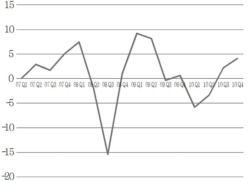
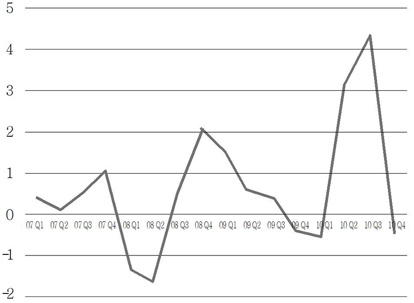
Next, the stationarity of the data was identified. The stationarity is the basic condition of ARIMA analysis, and is characterized by that the mean is constant, that variance of a constant should exist, and that autocovariance between two time points should depend on a time lag alone (Song Kyong-jae et al., 2005). As a result of estimating the trends by a unit root test, It was found that there were trends both for Seoul and Busan (p-value = 0.7478 (Seoul), 0.9145 (Busan)). To remove the trends from both regions, differencing was applied sequentially. In the case of Seoul, a stationary time series could be obtained from the first difference (Fig. 2), and in the case of Busan, a stable time series could be obtained from the second difference. (Fig. 3).
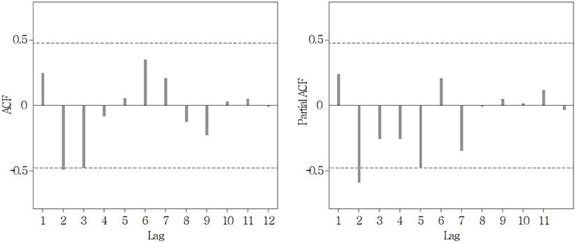
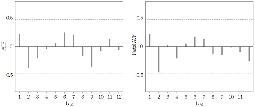
Lastly, the auto-correlation function (ACF) and the partial auto-correlation function (PACF) were used to identify the ARIMA model. As shown in Fig. 4 and Fig. 5, both ACF and PACF for Seoul and Busan show sinusoidal waves of decreasing amplitude, and showed no significant lag. As also shown in the results of Table 4, the p and q values of the ARMA (p, q) model for both regions represent 0.
After taking all the above results into consideration, ARIMA (0, 1, 0) model was selected for Seoul, and ARIMA (0, 2, 0) model for Busan, respectively.
The root mean square prediction error (RMSPE) value and the average rank value were used to compare the forecasting performance of the BMS model and the BMA model, together with the ARIMA models obtained above. The RMSPE value is the standard deviation of differences between observed values and predictive values, and was used to compare the accuracy of the models. And the average rank value is a value obtained by ranking the most excellent model at every forecasting time point and averaging them, and was used to derive and compare the most preferred models during the forecasting period. In addition, it was used as objective data in evaluating derived models by calculating the optimum number of variables used in the BMS model and the BMA model.
IV. Results of Analysis
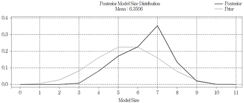
In Seoul, it was found that the probability was the highest when about 6.3506 variables on average were used in the posterior model (Fig. 6). As for the posterior model that satisfies Occam’s Window, a total of five were selected when the C value was 10, and a total of 7 were selected when the C value was 20 and 30. Among them, model 400, which used as its variables the fluctuation of land price (Seoul), the consumer price index, the market interest, the mortgage rate, and the CD rate, was selected as the best forecasting model with the probability of 5.64% (Table 5). Besides, in the other top-ranked models were included the combinations of the fluctuation of land price (Seoul), the consumer price index, the market interest, the mortgage rate, GDP (nominal), and GDP (real); and particularly in the case of Seoul, it was found that variables of demand play an important role in the prediction of the apartment sale price index.
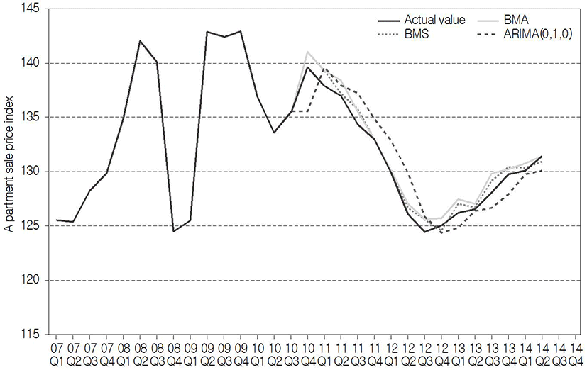
The results of the out-of-sample prediction of the apartment sale price index for Seoul from 1Q 2011 to 4Q 2014 are plotted on a graph, as shown in Fig. 7. To look at the apartment sale price index of Seoul during the period of analysis, basically, it is found that the range of fluctuation in the index value is relatively great between 2006 and 2013. It can be seen that the fluctuation is particularly severe from 3Q 2008 to 4Q 2010, and it represents the effects of the United States subprime mortgage crisis from 2008, which seems to have also influenced Korea’s recession and the shrinkage of consumer sentiment, and have in turn had a bad influence on the real estate market. It may be said that this phenomenon agrees with the above results of this study that variables of demand were used as variables of major models. As a result of comparing the forecasting performance between BMS, BMA, and ARIMA (0, 1, 0) by means of the root mean square error (RMSE) value, it was found that BMS and BMA of 0.747 and 0.967 (0.937), respectively, forecasted with small ranges of error, compared with ARIMA (0, 1, 0), which showed the value of 2.021, and that BMS showed the most excellent forecasting performance among them (Table 6). In addition, as a result of comparing the forecasting performance of the three models by means of the average rank value, BMS with the value of 1.3 was selected as the best model over all the intervals. From these results, it was seen that BMS having five values is a more suitable model than BMA, which considers eight values, on the basis of the above results that the optimum number of variables is 6.3506.
| BMS | BMA | ARIMA(0,1,0) | ||
|---|---|---|---|---|
| C=10 | RMSE | 0.747 | 0.967 | 2.021 |
| Average Rank | 1.3 | 2 | 2.7 | |
| C=20, 30 | RMSE | 0.747 | 0.937 | 2.021 |
| Average Rank | 1.3 | 2 | 2.7 |
2) Busan
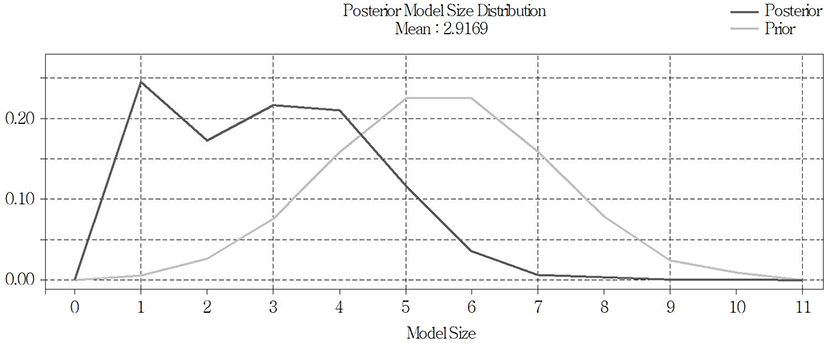
In the case of Busan, it was found that the posterior probability of models consisting of 2.9169 variables, which are comparatively fewer than Seoul, was the highest (Fig. 8). In case that C value was 20 and 30, it was found that a total of two models satisfied the Occam’s Window, and that of the two, model 10, which used GDP (nominal), was selected as the best forecasting model (Table 7). The other model 448 included the fluctuation of land price (Busan), the market interest, and GDP (real). In case that C value was 10, it was found that only model 10 satisfied the Occam’s Window.
| C value | Model name | Variable used | Probability |
|---|---|---|---|
| 10 | 10 | GDP (nominal) | 0.2424471 |
| 20, 30 | 10 | GDP (nominal) | 0.2424471 |
| 448 | Fluctuation of land price (Busan), market interest, GDP (real) | 0.0167098 |
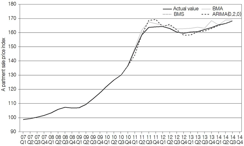
Similarly, the results of the out-of-sample prediction of the apartment sale price index for Busan, using the above models, are plotted in Fig. 9. In the case of Busan, it is found that fluctuation in the apartment sale price index during the same period is not severe, compared with Seoul, but increases steadily; and that the forecasting results also predicted the actual value better than the results for Seoul. As a result of comparing RMSE for the comparison of respective forecasting performance, it was found that, unlike Seoul, the forecasting performance was most excellent in BMA (2.054 (2.051)), followed by BMS (2.054), and ARIMA (0, 2, 0) (2.350). In terms of the average rank value, it was found that the forecasting performance of ARIMA(0, 2, 0) was the most excellent with the value of 1.4 (1.8) over all the intervals (Table 8). In Busan, it was found that BMA consisting of four variables was a more suitable model than BMS consisting of only one variable, also on the basis of the fact that the optimum number of variables is 2.9161.
| BMS | BMA | ARIMA(0,1,0) | ||
|---|---|---|---|---|
| C=10 | RMSE | 2.054 | 2.054 | 2.350 |
| Average Rank | 1.6 | 1.6 | 1.4 | |
| C=20, 30 | RMSE | 2.054 | 2.051 | 2.350 |
| Average Rank | 1.9 | 2.3 | 1.8 |
V. Conclusion
This study suggested the best analysis model for each region through the BMS and BMA methodologies that reflected the problem of uncertainty arising from the use of the existing methodologies, and showed that they can improve forecasting performance by comparative analysis with the AR model that has been used as the existing methodology. As a result of analyzing by region the posterior probability of 2,047 models consisting of the combinations of 11 variables, based on data from 1Q 2007 to 4Q 2010, it was found that for Seoul, the model using the fluctuation of land price (Seoul), the consumer price index, the market interest, the mortgage rate, and CD rate showed the highest probability, while for Busan, the model consisting of GDP (nominal) showed the highest probability; and a group of top-ranked models for each region were derived by using the Occam’s Window.
As a result of forecasting the apartment sale price index for a total of 16 quarters from 1Q 2011 to 4Q 2014, using models selected through BMS and BMA, it was found that their forecasting performance was more excellent in Busan that showed a relatively small range of fluctuation. As a result of using the average rank and MSE between the actual apartment sale price index and predicted values, the forecasting performance varied with the regions. First, in the case of Seoul, both RMSE and the average rank show the same results in the order of BMS, BMA, and ARIMA. In the case of Busan, there was differences between RMSE and the average rank; as for RMSE, the forecasting performance was most excellent in BMA, followed by BMS and ARIMA, while as for the average rank, the forecasting performance was most excellent in ARIMA, followed by BMS and BMA. This implies that basically, BMS and BMA are superior in the medium-and long-term prediction of the apartment sale price index for Seoul that shows a wide range of fluctuation, and that they are also excellent in the short-term prediction for Busan that shows a small range of fluctuation. In the case of Busan, it was found that the longer the period of prediction, the more excellent the ARIMA; which seems to be because the BMS model and the BMA model selected from data on the first 20 quarters are advantageous to short-term analysis, but fail to reflect information agreeing with a prolonged period in the long-term analysis.
The contributions made by this study can be viewed largely in three respects. First, the methodologies suggested by this study improved the problem of the uncertainty of model selection arising in the existing studies. As for the existing econometric approaches, they can improve forecasting performance according as they consider more variables, but at the same time they may be faced with the problem of overfitting, and should undergo separate testing procedures to identify correlations between variables. In contrast, this study has the advantage that all variables can be considered without the overfitting problem and separate testing because each probability and uncertainty arising from variable selection are basically reflected in advance.
Further, it did not rely on one model alone, but considered all models probabilistically, and thus improved forecasting performance, compared with the existing approaches. In the existing studies, information loss occurs because they select and consider one model consisting of specific variables among numerous factors that influence housing price. In contrast, the Bayesian framework suggested by this study can conduct analysis with more information than the existing approaches and derive forecasting results with a narrower range of error because it probabilistically considers all models consisting of the combinations of every variable in its analysis.
In addition, this study suggested analysis models and results that reflect regional characteristics, by comparing and analyzing BMS and BMA according to regions. According to the existing studies, it is very important to consider regional characteristics in developing an analysis model, for regional factors have great effects on housing price. On this, this study was able to derive and select models suitable for individual regions by comparatively analyzing Seoul, which showed a relatively great range of fluctuation, and Busan, which showed a relatively small range of fluctuation.
2. Limitations
This study has significance in that it derives a more improved model of housing price analysis, using the Bayesian approach that reflects the uncertainty of model selection. However, it has some limitations in other respects. First, it failed to reflect the empirical analysis of effects on actual housing price, for it focused only on macroeconomic factors, not a number of hedonic factors that have immediate effects on housing price; which led to the result that the models selected for Seoul and Busan did not represent their regional characteristics well. But this study preferentially considered the use of macroeconomic variables that enable easy data collection and generalization, for the primary objective of this study was to suggest a new forecasting model given model uncertainty and to show its superiority in forecasting performance to the existing approaches. It is deemed that future studies may be able to improve this problem by more practical housing price forecasting through BMS and BMA analysis using hedonic factors at the levels of “gu” and “dong” and macroeconomic factors.
In addition, the problem may occur that the best models derived in this study do not best fit actual prediction. As for BMS and BMA, the kind and number of their best models vary according to the number of variables used by a researcher and the period of analysis. Therefore, in case of forecasting the apartment sale price index at this point in time, the future price should be predicted with all available data; however, this study used a few random data for comparative analysis, and thus there occurs differences between the models of this study and the best models in actual prediction. That is, models selected by this study may be viewed as best models derived for a specific period to show the improvement of forecasting performance due to reduction in model uncertainty, and models suitable for actual prediction can be selected by adjusting the period of analysis.


